Brain Imaging - Variability
Variability, replication, and longitudinal studies
One of our main areas of research is Statistical methods for the analysis of populations of brain images. Expertise includes fMRI, structural MRI (T1, T2, FLAIR, PD, etc), SPECT, CT. Areas of applications include Attention Deficit Hyperactivity Disorder (ADHD), Multiple Sclerosis (MS), Alzheimer disease (AD), brain cancer, Traumatic Brain Injury (TBI), and Stroke. Our brain imaging collaborators include Daniel Reich, Peter Calabresi, Susumu Mori, Jerry Prince, Alfredo Quinones-Hinojosa, Jim Pekar, John Krakauer, Brian Schwartz, Peter van Zijl, Dzung Pham, Susan Spear-Bassett and Stewart Mostofsky.
Three main areas areas of expertise include variability decomposition and modeling, association and prediction, and translational neuroscience. Here we provide an overview of methods and data sets for modeling and analyzing variability decomposition with special emphasis on replication and longitudinal studies.
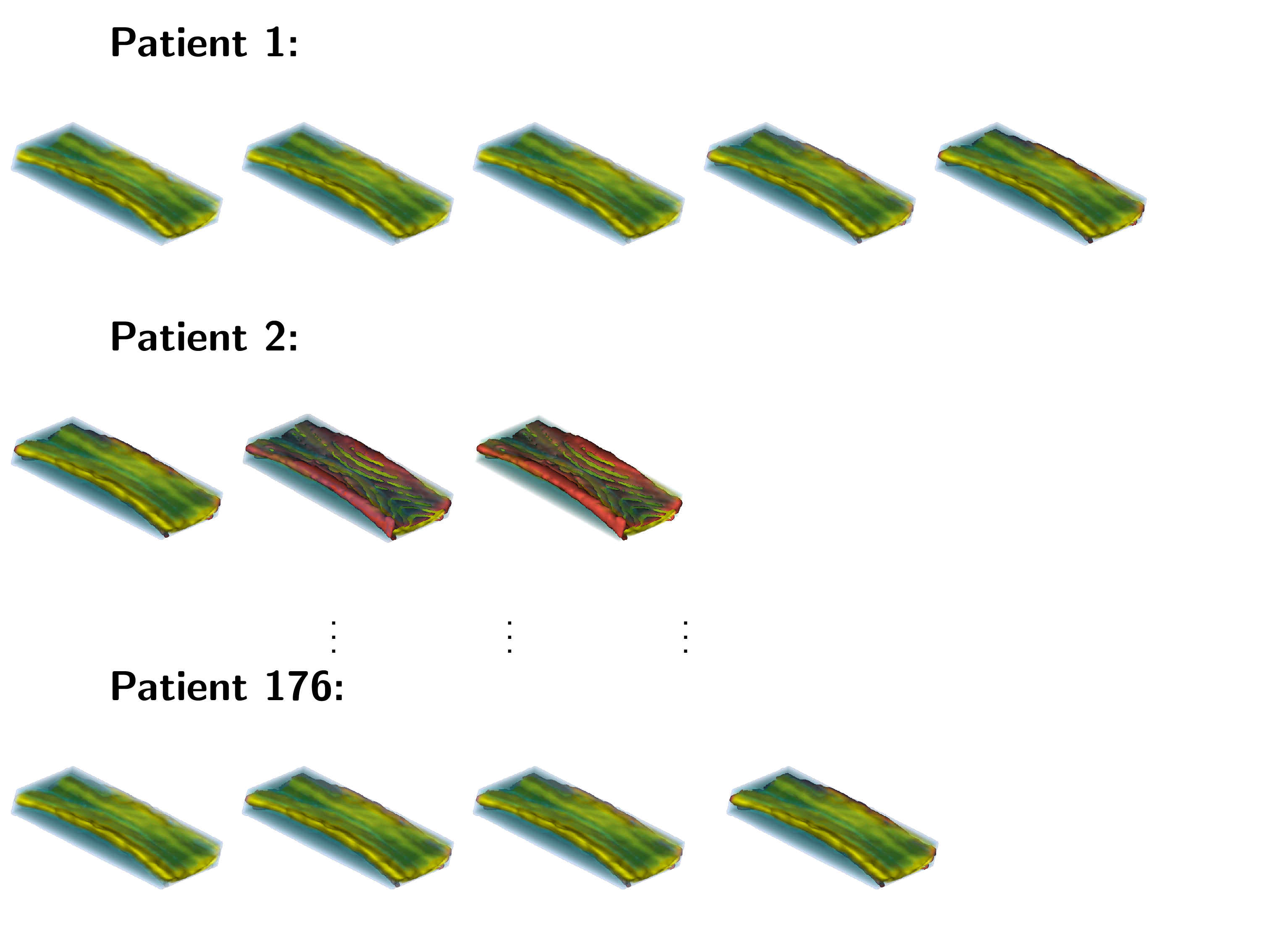
Variability decomposition is a classical problem in Biostatistics concerned with reasonably apportioning variability to known sources. For example, brain imaging replication or longitudinal studies require identifying the size and type of variability due to subject, visit, time, etc. We have developed a suite of methods for the analysis of such data. These methods are based on principal component approaches and include:
- multilevel functional principal component analysis (MFPCA) with its high dimensional counterpart (HD-MFPCA) for replication studies. This is a main tool for studying reliability of replication studies and is especially useful for characterizing and visualizing the type of replication error;
- longitudinal functional principal component analysis (LFPCA) with its high dimensional counterpart (HD-LFPCA) for populations of images observed at multiple visits; and
- structural functional principal component analysis (SFPCA) with its high dimensional counterpart (HD-SFPCA) for data with known complex-by-sampling-design data.
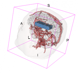
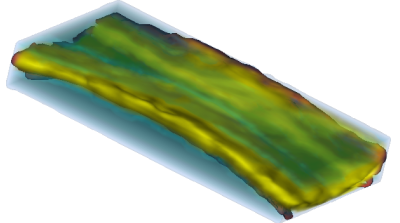
An example of data that inspired such models is shown below. This is a longitudinal study of fractional anisotropy (a measure of how "directed" is the water movement, which is thought to be a proxy for detailed anatomy, such as white matter bundles) along the corpus callosum (the most easily recognizable white matter tract in the brain; corpus callosum is part of the blue right rectangular prism shown in the picture above.) The fractional anisotropy of the corpus callosum can be represented using color around the 3D corpus callosum (a folded-carpet-like white matter bundle that connects the two hemispheres) with red indicating higher and green indicating lower fractional anisotropy. The image below is a 4D (fourth being color) of the corpus callosum of one subject at one visit. We left a blue hue around it to better relate it to the previous image.
For fMRI (and other type of images that can be represented as matrices) we have developed Population Value Decomposition (PVD), a method for the analysis of population of images. The method is similar to the ultra popular singular value decomposition (SVD) which decomposes one (subject-specific) matrix. In the case of data analysis one is often faced with many matrices (e.g. fMRI images) and focus is both on dimensionality reduction and modeling and prediction of the subject-specific information. Thus, PVD starts with a set of subject-specific matrices Yi which is T by V dimensional (e.g. time by voxel in fMRI studies) and decomposes them as Yi = PViD + Ei, where P is T by A matrix, Vi is an A by B matrix, D is A by V dimensional, and Ei is a T by V matrix of residuals. In this formulation, the P and the D matrices are population-specific, which allows the entire variability in the data to be explained by the subject specific, not-necessarily diagonal, inner matrix Vi. If either T or V or both are very large but A and B are small to moderate then super complicated problems related to ultra high dimensional data can easily be handled in the much smaller sub-space spanned by the Vi matrix. In particular, any linear model on Vi (that is, on the subject-specific coefficients) has an immediate counterpart in the original data space spanned by Yi. PVD does not require the P and D matrices to be orthogonal, though the fast default PVD approach ensured orthonormality. This is esecially useful if one has some knowledge about the data and the matrices P and D can be constructed using, for example, splines, Fourier, wavelets bases. Once the model is fitted inspecting the residuals Ei can be done, which may suggest lack of fit, better models, and alternative ways of approaching the problem.
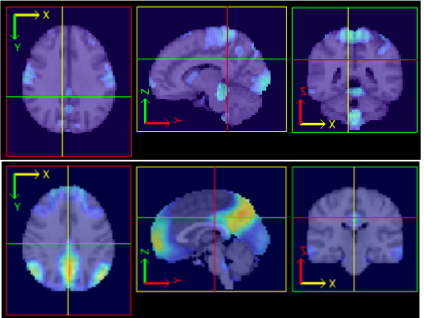
As an example, the following plots show PVD fits to fMRI paradigm related data from a study of subjects at risk for Alzheimer''s disease versus controls.
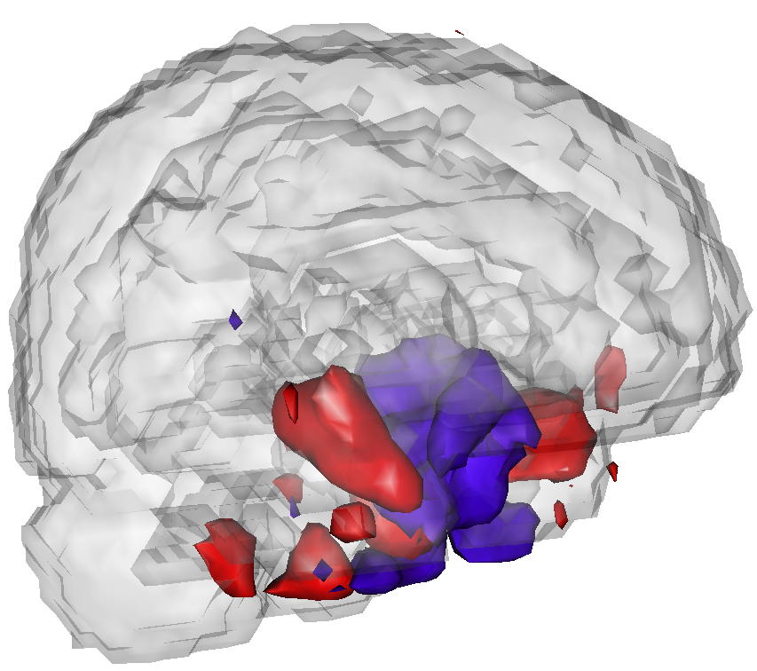
These areas appear to predict risk stats and subsume important components of brain anatomy that have shown previous associations with AD.
A related collection of work considers variation as measured by so-called independent components analysis (ICA). Group ICA for fMRI is frequently used to discover brain networks via sychronous spontaneous BOLD resting state flucuations. The picture below illustrates the concept behind group ICA.
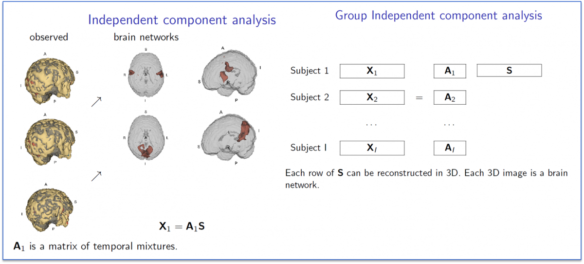
In Ani Eloyan's work, she has developed a novel new ICA algorithm and extended it to high dimensional settings. She has applied this algorithm to the NITRC 1,000 Connectome data and below we show images of the motor and default mode network.
