Biosignals
Biosignals is a word that we invented to cover a wide range of applications in Statistics. It was originally intended to describe data that are collected from humans and animals using non-invasive sensors, such as electric leads, microphones, video recordings, etc. Once we started analyzing ECoG data, which is obtained directly from hundreds of electrodes sitting on the surface of the brain after the skull is surgically removed, we were compelled to drop the "non-invasive" label. Thus, we currently define a Biosignal to be a "uni- or multivariate time series of measurements aquired from a vertebrate animal and is a reasonable proxy for an underlying biological process."
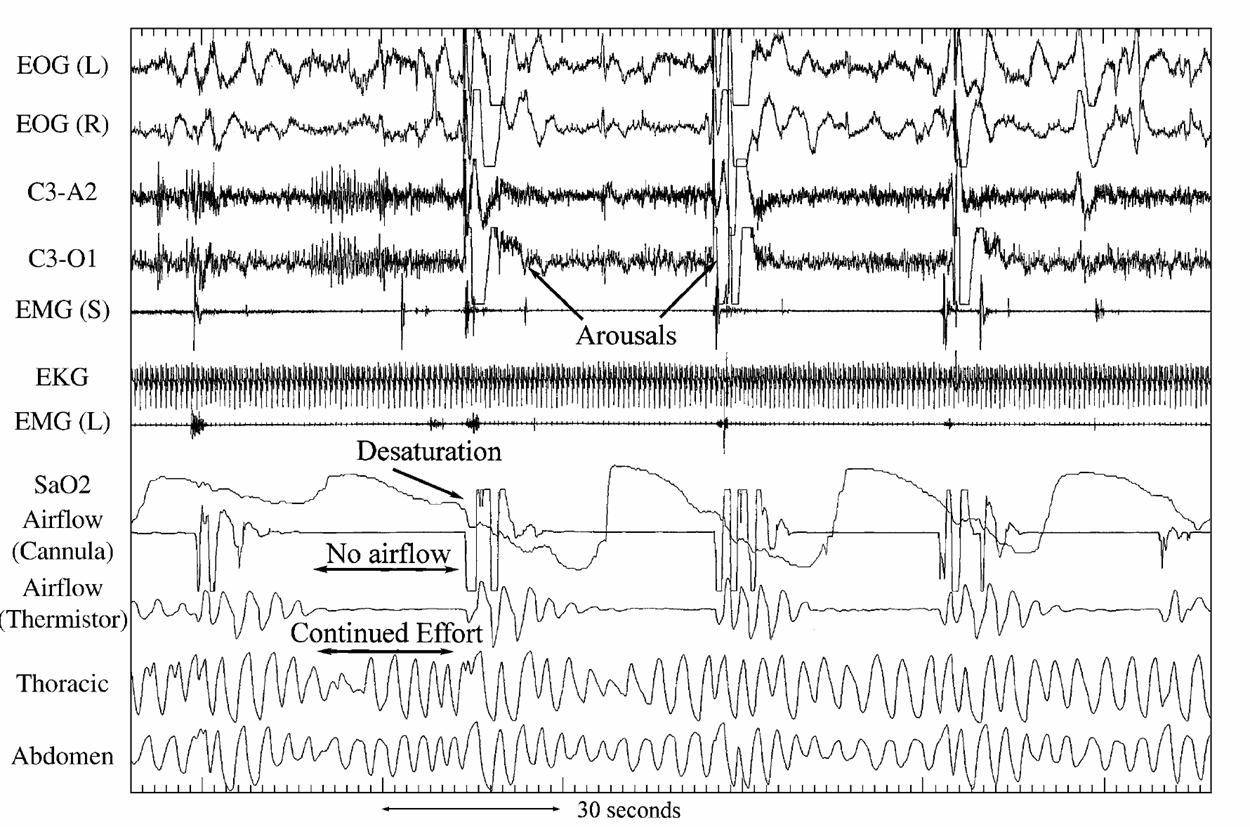
There are many types of Biosignals and studies. Our group has been involved in several types of studies involving populations of Biosignals. Here we provide some background on studies conducted by our group that involve Biosignals. One of the first studies is the Sleep Heart Health Study (SHHS) led by our close collaborator, Naresh Punjabi. The SHHS collected sleep studies at two visits, roughly 5 years apart, for thousands of subjects. A sleep study consists of a polysomnogram (PSG) is a quasi-continuous multi-channel recording of physiological signals acquired during sleep that include two surface electroencephalograms (EEG), electrocardiogram (EKG), electromyogram (EMG), and electrooculogram (EOG). Below we show a 3 minute snapshot PSG for one subject indicating the quasi-continuous nature of the recording. For more information of our group's work on this type of data check out our papers.
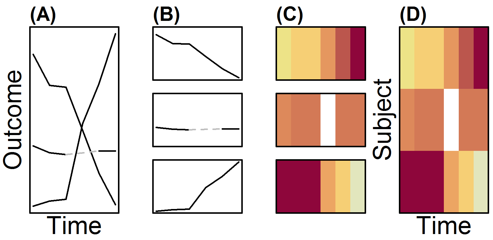
These data are further classified visually into rapid eye movement (REM) sleep or one of four non-REM (NREM) sleep stages. Traditionally, sleep stages are visualized with a hypnogram, a discrete-state discrete-time trajectory. Hypnograms of many individuals over time on the same plot form a "spaghetti plot", and as such are prone to overplotting. The overplotting hinders their effective use in visualizing the data from population-level sleep studies. Our group advocates the use of lasagna plots in instances like these. The figure below describes the process of making lasagna plots from spaghetti plots by, essentially, making "noodles into layers". From left to right, (A) a spaghetti plot with 3 noodles where trajectories overlap. B, Extracting each noodle representing repeated measures on a subject, (C) a layer is made by letting color represent the outcome (red low, orange moderate, yellow high). (D), Individual layers are then stacked to make a lasagna plot, with no overlapping of subject information.
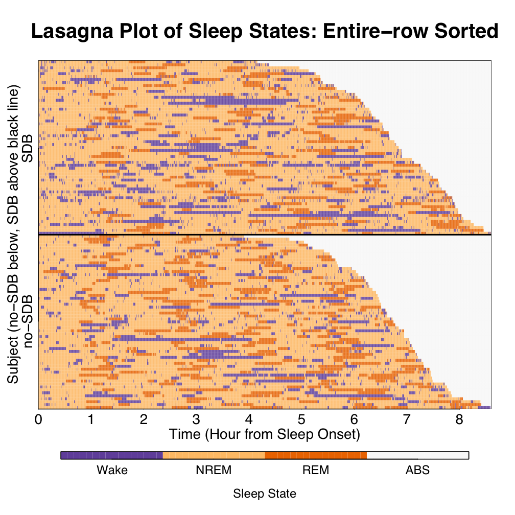
A hypnogram works well for 1 subject, as used in doctor-patient care. For epidemiological studies, overplotting is apparent for a modest study of 118 subjects. A lasagna plot prevents overlapping and the layers sorted according to group status and total sleep time conditional on group status. Lasagna plots were first introduced by Bruce Swihart as a "saucy alternative to spaghetti plots."
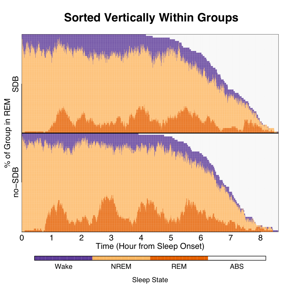
For a group-level look at temporal trends, sorting of states within the columns of time conditional on group status can be conducted. Results of such a sorting are shown below. Interestingly, whether before patterns were quite hard to recognize, after sorting patterns start to emerge.
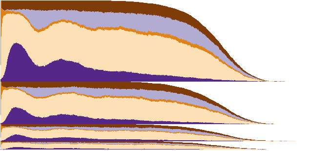
In the previous figure, 2 groups of 59 subjects each were displayed for 3-state sleep. Below we display 4 groups of SDB severity for a total of 5600 subjects for 5-state sleep. The plot is sorted within group within time, giving a look at the group-level temporal evolution of Slow-wave (deep) sleep. The "break-out" and equal scaling of the four groups are depicted for ease of view. From the figures, SDB severity might dampen the Slow-wave biosignal. Keep in mind the slow-wave biosignal information is obscured using fewer states, fewer groups, and fewer subjects.
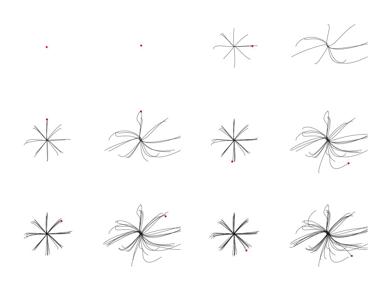
The number and diversity of observed biosignals is incredible, which provides unprecedented opportunities for Biostatisticians. For example our collaborator, John Krakauer, is interested in understanding the effect of stroke on motion integrity. In an experiment designed to understand kinematic similarities and differences between healthy controls, mildly affected stroke patients, and severely affected stroke patients, subjects were asked to reach toward eight targets in a two-dimensional planar motion task. Below we show motions made by two subjects, each of whom suffers from mild stroke affecting their dominant arm. The subjects exhibit vastly different motor abilities for relatively similar brain injuries." Jeff Goldsmith is leading the modeling and analytic efforts of our research group for this type of data.
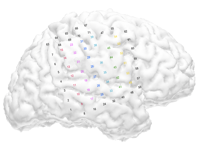
A much cleaner electric signal can be obtained directly from the brain of people who undergo brain surgery. In this case a mesh of 71 leads was placed directly onto the brain of a person whose skull was removed. Electrical signals obtained directly from the brain is referred to as Electrocorticography (ECoG) to differentiate it from Encephalography (EEG), which record electrical signals obtained without removing the skull.
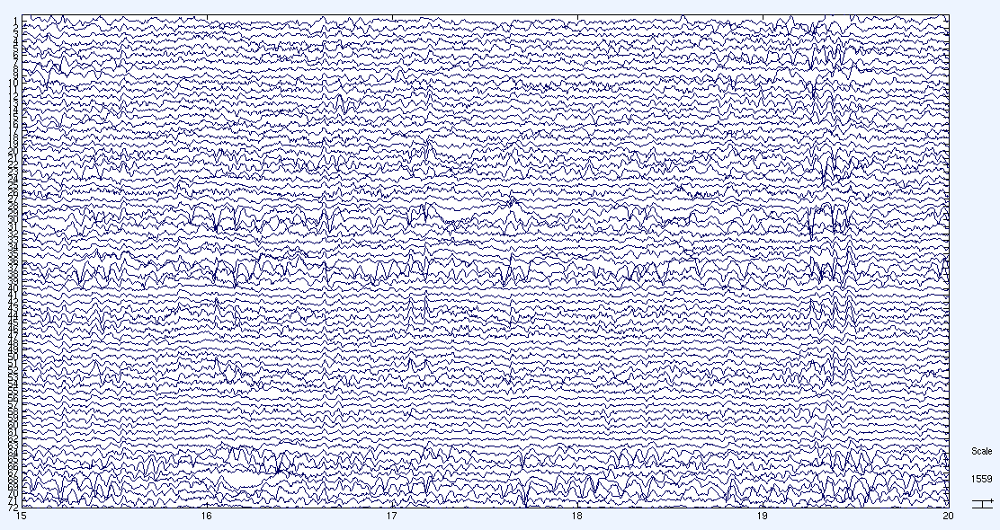
ECoG data are sampled at much higher frequency than EEG data (2,500Hz versus 150Hz) and produce very dense time series. The plot below provides a foretaste (scary or not?) of what the actual data look like in a 5 second interval (~1,000,000 data points over 71 channels). Each row is a electrical signal from one channel (there are 71 rows). One of the problem Haley Hedlin worked on was to find Granger causality among these time series. Granger causality is essentially trying to quantify which time series (channels) fire first, second, etc. This is a rather difficult problem as there is no obvious way of solving the problem.
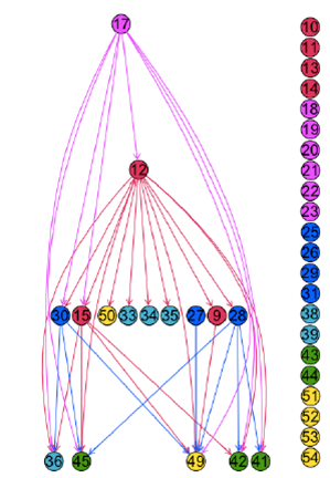
After some pretty neat statistical analysis the following temporal tree was identified. The interpretation is that time series activity observed in channel 12 tends to be preceded by observed activity in channel 17, and so on.

